
A little over two years ago, while exploring the edX platform for online courses, I came across a fantastic one about programming for beginners called Nature in Code: Biology in JavaScript. This course shows how basic programming constructs can be used as a powerful tool to describe, understand and reason about our natural world.
In this post, we'll look at how the aforementioned course teaches and translates scientific ideas such as evolution and epidemics, using simple models, into code. As a starting point, we define a null model, then we look into how mutation and migration (two of the main forces that lead to evolution) are implemented. And then, building from the previous ideas, we will briefly touch on how the spread of infectious diseases can be represented in code.
The Hardy-Weinberg Model
In biology, evolution is the change in genetic composition of a population over time. The course identifies four forces that lead to this change: - natural selection, as described by Charles Darwin, where individuals with characteristics best suited to their environment are more likely to survive, reproduce and pass their genes onto their children1 - genetic drift, where the change in genetic composition is due to random chance - migration, which refers to population moving from one place to another - mutation, which is described as the ultimate engine of diversity creation.
The course introduces the Hardy-Weinberg Model - also known as the null model, as being the model that describes how a system would behave without any of the forces of interest.
It relies on the following simplifying assumptions: - an infinite population size - non-overlapping generations - sexual reproduction happens randomly - and none of the four forces above is in action
Let's consider a basic model of a gene declined into two alleles a1 and a2. A gene is defined as the basic physical and functional unit of heredity.2 Every gene exists in multiple versions, called alleles, and these versions are the ones that make us unique.
For example, the human eye colour is predominantly determined by two genes, OCA2 and HERC2. This last gene comes in two versions, the C and the T alleles. The combination of those two alleles is what will (mostly) determine an individual's eye colour. A person with two copies of the C allele will likely have blue eyes (72% probability). One with two copies of the T allele will likely have brown eyes (85% probability). And one with both alleles will have brown eyes with a 56% probability.
Going back to our basic model, we'll consider the Hardy-Weinberg allele frequencies f(a1) as p and f(a2) as q to not change over time. And the resulting genotype frequencies - f(a1a1), f(a1a2) and f(a2a2) - may vary within one generation, and then stabilise and never change again over time.
In JavaScript, these Hardy-Weinberg frequencies are initialised as follows:
// generation 0 genotype frequencies
let a1a1 = 0.15;
let a2a2 = 0.35;
let a1a2 = 1 - (a1a1 + a2a2);

// allele frequencies (constant over time)
const p = a1a1 + (a1a2 / 2);
const q = 1 - p;
Calculating the Hardy-Weinberg model over 20 generations (for example):
function hardy_weinberg_model() {
    for (let gen = 1; gen <= 20; gen++) {
        next_genotype_generation();
        console.log("generation", gen, ":", a1a1, a2a2, a1a2);
    }
}

// calculate next generation data
function next_genotype_generation() {
    a1a1 = round(p * p, 2);
    a2a2 = round(q * q, 2);
    a1a2 = 2 * round(p * q, 2);
}

// round a given number to n digit after the decimal point
function round(value, n) {
    const shifter = Math.pow(10, n);
    return Math.round(value * shifter) / shifter;
}
When the simulation above is run, generation after generation, the Hardy-Weinberg genotype frequencies do not change as the allele frequencies remain constant.
Mutation: The Power Of Mistakes
Mutation is the change in genetic sequence, and is the main cause of diversity among organisms. It generally happens during cell replication, which is the process during which a given cell will produce two identical replicas of its own DNA. It is during this process that a small change - a small error - might occur leading to mutation in one of the new cells. Although this (kind of) mistake is very rare, it manifest itself as random mutation.
To implement this idea in JavaScript, as the DNA molecule is formed of four bases - adenine, guanine, cytosine, and thymine - we use an array to store a DNA sequence as a sequence of the four bases. For example, for an individual, we'll represent their DNA sequence as [A, G, C, C, A, T]. Then, we represent a whole population as a two-dimensional array of similar sequences. As we'll be looking into changes in population over time, this leads to a 3D array where the third dimension is time.
Assuming we start with an identical population, our first generation (before mutation) can therefore be calculated as follows:
const BASES = ['A', 'G', 'C', 'T'];
const number_of_sequences = 100;
let sequences = []; //population array
let original_sequence = [];

function first_generation() {
  first_sequence();
  for (let i = 0; i < number_of_sequences; i++) {
    sequences.push(original_sequence.slice());
  }
}
where first_sequence() is a function that generates the original sequence, and we copy this sequence a hundred times.
const sequence_length = 20;

 // generating original sequence
function first_sequence() {
  for (let i = 0; i < sequence_length; i++) {
    original_sequence.push(random_base(""));
  }
}

// generating a random choice from the four DNA bases characters
function random_base(current_base) {
  let index;
  let new_base;

  do {
    index = Math.floor(Math.random() * 4);
    new_base = BASES[index];
  } while (new_base === current_base);

  return new_base;
}
Now that we have a first generation, mutation will be expressed as a random phenomenon over time, with a very low mutation probability of 1/10000 to translate its rarity. Running this simulation over a hundred generations, we get:
const mutation_rate = 0.0001; // per base and generation
const number_of_generations = 100;

// mutation model
function run_generations() {
  for (let i = 0; i < number_of_generations; i++) {
    // for each generation | current generation is i
    for (let j = 0; j < sequences.length; j++) {
      // for each sequence | current sequence is sequences[j]
      for (let k = 0; k < sequences[j].length; k++) {
        // for each base | current base is sequences[j][k]
        if (Math.random() < mutation_rate) {
          sequences[j][k] = random_base(sequences[j][k]);
        }
      }
    }
  }
}
A log of the results to the console looks like this:
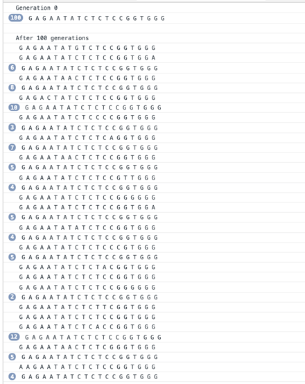
So, even a very low mutation probability will result in a significant increase in diversity over time.
Migration: Spatial Models
In studying migration, we build from the Hardy-Weinberg model, considering diploid individuals (having two copies of genetic material), but relax two of our previous simplifying assumptions. - First, we no longer consider to have an infinite population size. - Second, we are no longer assuming random sexual reproduction. Instead, we consider where individuals are in space. So, when mating, it's much more likely that an individual will choose a close-by partner, rather than an individual who is far away.
Relaxing these two assumptions gives us a spatial model.
We represent such a model with a finite grid, where each cell contains an individual. And we add a rule about mating distance: for each individual in the grid, we define a maximum mating distance. For example, if we set such a distance to 1, an individual in the middle of the grid will have eight possibilities in choosing a partner.
When implementing this model, we start with allele frequencies, and grid initialisation, and we set our maximum mating distance to 1.
// spatial model initialisation
const grid_length = 100;
const p = 0.5; // p is allele a1 frequency
const grid = [];
const max_mating_distance = 1;

// generation 0 genotype frequencies
let a1a1 = 0;
let a1a2 = 0;
let a2a2 = 0;
let generation_counter = 0;
Then, we randomly assign individuals in the grid:
function init_grid() {
    for (let i = 0; i < grid_length; i++) {
        grid[i] = [];
        for (let j = 0; j < grid_length; j++) {
            let random_num = Math.random();
            if (random_num < p * p) {
                grid[i][j] = "A1A1";
                a1a1++;
            } else if (random_num > 1 - ((1 - p) * (1 - p))) {
                grid[i][j] = "A2A2";
                a2a2++;
            } else {
                grid[i][j] = "A1A2";
                a1a2++;
            }
        }
    }
}
Once we have our population initialised, we look at what happens generation after generation. In other words: - each individual chooses a mating partner in accordance with the maximum mating distance defined earlier - then we generate the children given the parents' genotypes, and store them in a temporary grid - and finally, once we've run through all the individuals, we replace the parent generation with the offspring generation.
function pick_mating_partner(position_i, position_j) {
  let x = random_value_between(position_i - max_mating_distance, position_i + max_mating_distance);
  let y = random_value_between(position_j - max_mating_distance, position_j + max_mating_distance);
  x = bounded_index(x);
  y = bounded_index(y);
  return grid[x][y];
}
In the above snippet of code, bounded_index refers to a function that wraps around the grid (when necessary), and the random_value_between returns a random value between two given values.
The function that generates the offspring once the parents' genotype is known can be broken down as follows: - when both parents are of the same genotype, then, as one would expect, the offspring will be of the same genotype - when the first parent is homozygous (identical alleles), and the other is heterozygous, a randomly generated probability determines which parent's genotype the child fully inherits from - when both parents are homozygous, but of different genotypes, a randomly generated probability determines whether the child is homozygous or heterozygous.
function get_offspring(parent1, parent2) {
    let probability = 0;

    if (homozygous_and_identical(parent1, parent2)) {
        return parent1;
    }

    if ((homozygous(parent1) && heterozygous(parent2))
            || (heterozygous(parent1) && homozygous(parent2)) {
        probability = Math.random();
        if (probability < 0.5) {
            return homozygous_genotype_from(parent1, parent2);
        } else {
            return "A1A2";
        }
    }

    if (homozygous_non_identical(parent1, parent2)) {
        return "A1A2";
    }

    if (heterozygous_and_identical(parent1, parent2)) {
        probability = Math.random();
        if (random_num < 0.25) {
            return "A1A1";
        } else if (random_num > 0.75) {
            return "A2A2";
        } else {
            return "A1A2";
        }
    }
}
The intermediate helper functions are as simple as the following:
// are parents homozygous and identical
function homozygous_and_identical(parent1, parent2) {
    return (identical(parent1, parent2) && parent1 === "A1A1")
          || (identical(parent1, parent2) && parent1 === "A2A2");
}

// are parents homozygous but not identical
function homozygous_non_identical(parent1, parent2) {
  const non_identical = ! identical(parent1, parent2);
    return (non_identical && is_heterozygous(parent1))
          || (non_identical && is_heterozygous(parent2));
}

// are both parents heterozygous
function heterozygous_and_identical(parent1, parent2) {
    return identical(parent1, parent2) && parent1 === "A1A2";
}

function homozygous(parent) {
    return parent === "A1A1" || parent === "A2A2";
}

function heterozygous(parent) {
    return parent === "A1A2";
}

// are parents of the same genotype
function identical(parent1, parent2) {
  return parent1 === parent2;
}

// return a homozygous genotype from a parent
function homozygous_genotype_from(parent1, parent2) {
    if (homozygous(parent1)) {
        return parent1;
    }
    return parent2;
}
The complete code for generating the migration spatial model and running a simulation over a 100 generations for example can be found here. And, with the help of D3 visualisation library, we can generate a visualisation of how this model will evolve over time.
Epidemics: The Spread of Infectious Diseases
Nature in Code, Biology in JavaScript concludes the course by looking into how infectious diseases spread in a population. And this last chapter is my favourite of the entire course as it shows how programming (and software in general) can be used as a powerful tool to understand and find solutions to real world problems such as those caused by infectious diseases.
Following the same modelling process as before, the course defines preconditions for an epidemic to occur: - a susceptible population - and an infectious agent that affects hosts and can get passed on to other susceptible hosts. However, all infectious agents do not necessarily cause illness in their hosts.
Those preconditions give way to a Susceptible-Infected-Recovered (SIR) model. Initially, individuals are considered to be susceptible to an infectious disease. When exposed to an infectious agent, with a certain probability they get infected, and can in turn infect other susceptible individuals. Finally, under certain conditions (modelled here as a probability), they clear the infection and are considered recovered.
These three stages of evolution can be implemented in code following the same steps as before. And that leads to a simulation that looks like this:
Finally, in implementing recovery, we discover under which conditions an infectious disease can be slowed down and eventually stopped.